1. Consider the bicycle racing problem in the presence of air resistance. Determine the terminal (ultimate) velocity analytically. How do you determine the terminal velocity numerically? Write down the numerical scheme for solving equations of motion using simple Euler's method.

Ans.:

The drag force be F_drag = - CrAv², where C is the drag coefficient, r is the density of air, and A is the frontal area of the object. Let P be the (constant) power output of the rider (P=Fv; F=P/v). Then the motion can be described by the equations

dx/dt =v

dv/dt = P/(mv)- (CrA/m)v²

The terminal velocity is reached when dv/dt=0 (the velocity no longer changes; it saturates). Thus

P/(mv)- (CrA/m)v²=0;

this leads to the terminal velocity: . Numerically, you can set an error tolerance, when dv/dt is less than the error tolerance, you can claim that the terminal velocity is reached.

Euler's method for solving these equations are based on the following updating scheme.

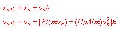
where h is the time step.

2. Temperature profile in a cup of coffee. A cup of coffee is warmed from the bottom with a fixed temperature T₀. If the room temperature is equal to T_e, construct a numerical scheme for obtaining the temperature profile inside the cup. Assume that the temperature inside the cup is uniform on a horizontal layer, but varies in the vertical direction. Write Matlab codes for obtaining the temperature profile and plot the result.

Ans.:

We can use a one-dimensional grid to discretize the height variable y. We can use N grid points (n=1 corresponds to the bottom surface of the cup and n=N corresponds to the top surface of the cup) and the following relaxation scheme to obtain the equilibrium temperature distribution:

The boundary conditions are:  and . We can set the interior temperatures to be zero at the beginning and iterate the above equation until temperature difference between two consecutive iterations at each grid point is smaller than a predefined error tolerance.

The Matlab codes for doing the temperature relaxation is given below:

N = input('Enter number of grid points ');
temp1 = input('Enter temperature at the bottom of the cup ');
temp2 = input('Enter room temperature');
tolerance = input('Enter equilibrium tolerance ');
%
% Initialize and print temperature matrix.
old = zeros(N,1);
old(1) = temp1;
old(N) = temp2;
disp('Initial Temperatures');
disp(old)
new = old;
equilibrium = 0;

%
% Update temperatures and test for equilibrium.
%
while ~equilibrium

  for n=2:N-1
    new(n) = (old(n-1) + old(n+1))/2;
  end

  if all(new-old <= tolerance)
    equilibrium = 1;
    disp('Equilibrium Temperatures');
    disp(new)
  end

  old = new;

end %while loop

plot(new)

3. Global weather forecasting. To do global weather forecasting, we need to solve the coupled partial differential equations for the temperature, velocity, and pressure, and other fields. To solve these differential equations numerically, we need to discretize the equations by using a spatial grid. If 1 million grid points are used to cover the Earth surface (the radius of the earth is about 6,400km), what is the typical distance between each grid point? Can you predict the local weather of Singapore with this model? If we use 1000 grid points in the vertical direction (for doing 3D modeling), the total number of grid points will be 1 billion. How much computer memory is needed to store a state of the system (we assume that each variable needs 8 bytes of memory for storage, and we only consider temperature, velocity, and pressure fields).

Ans.:

The area for a unit cell in the grid that covers the surface of the earth is about

(km² ) = 515 km²

The typical distance between two grid points is about  km.

In this case Singapore is only represented by a few grid points; the model can not be used to predict detail weather pattern in Singapore.

If 1000 grid points in the vertical direction is used, there will be total 1 billion grid points in the 3D grid. If we only consider temperature, velocity, and pressure field, the total number of variables need to be keep track of at each grid point is 5 (there are three components in each velocity). The number of bytes required to require all the information at each time step is

(billion bytes) 40 GBytes.